library(lmtest) # Dw test
library(ggplot2)
library(lubridate) # 날짜 다루는 패키지해당 자료는 전북대학교 이영미 교수님 2023고급시계열분석 자료임
패키지 설치
options(repr.plot.width = 15, repr.plot.height = 8)국내총인구
z <- scan("population.txt")
head(z)- 25012374
- 25765673
- 26513030
- 27261747
- 27984155
- 28704674
pop = round(z/10000)
head(pop)- 2501
- 2577
- 2651
- 2726
- 2798
- 2870
tmp.data <- data.frame(
 day = seq(ymd("1960-01-01"),by='year', length.out=length(z)),  #60년 1월 1일부터 연단위로, 데이터길이는 z와 동일하게.
 #day = 1959 + 1:length(z),
 pop = round(z/10000),
 t = 1:length(z),
 t2 = (1:length(z))^2
)
head(tmp.data)| day | pop | t | t2 | |
|---|---|---|---|---|
| <date> | <dbl> | <int> | <dbl> | |
| 1 | 1960-01-01 | 2501 | 1 | 1 |
| 2 | 1961-01-01 | 2577 | 2 | 4 |
| 3 | 1962-01-01 | 2651 | 3 | 9 |
| 4 | 1963-01-01 | 2726 | 4 | 16 |
| 5 | 1964-01-01 | 2798 | 5 | 25 |
| 6 | 1965-01-01 | 2870 | 6 | 36 |
시도표그리기
ggplot(tmp.data, aes(day, pop)) +
 geom_line(col='skyblue', lwd=3) +
 geom_point(col='steelblue', cex=3)+
 theme_bw() +
 #scale_x_date(date_labels = "%Y-%m") +
 theme(axis.title=element_blank(),    # ggplot 배경 변경
 axis.text= element_text(size=20))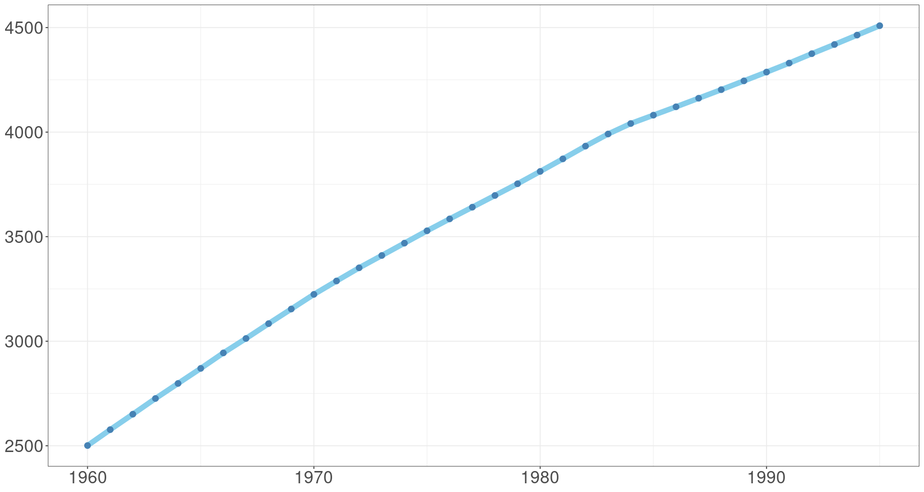
ggplot(tmp.data, aes(day, pop)) +
 geom_line(col='skyblue', lwd=3) +
 geom_point(col='steelblue', cex=3)+
 xlab("time") + ylab("Population")+
 theme_bw() +
 #scale_x_date(date_labels = "%Y-%m") +
 theme(axis.text= element_text(size=20),
 axis.title= element_text(size=30))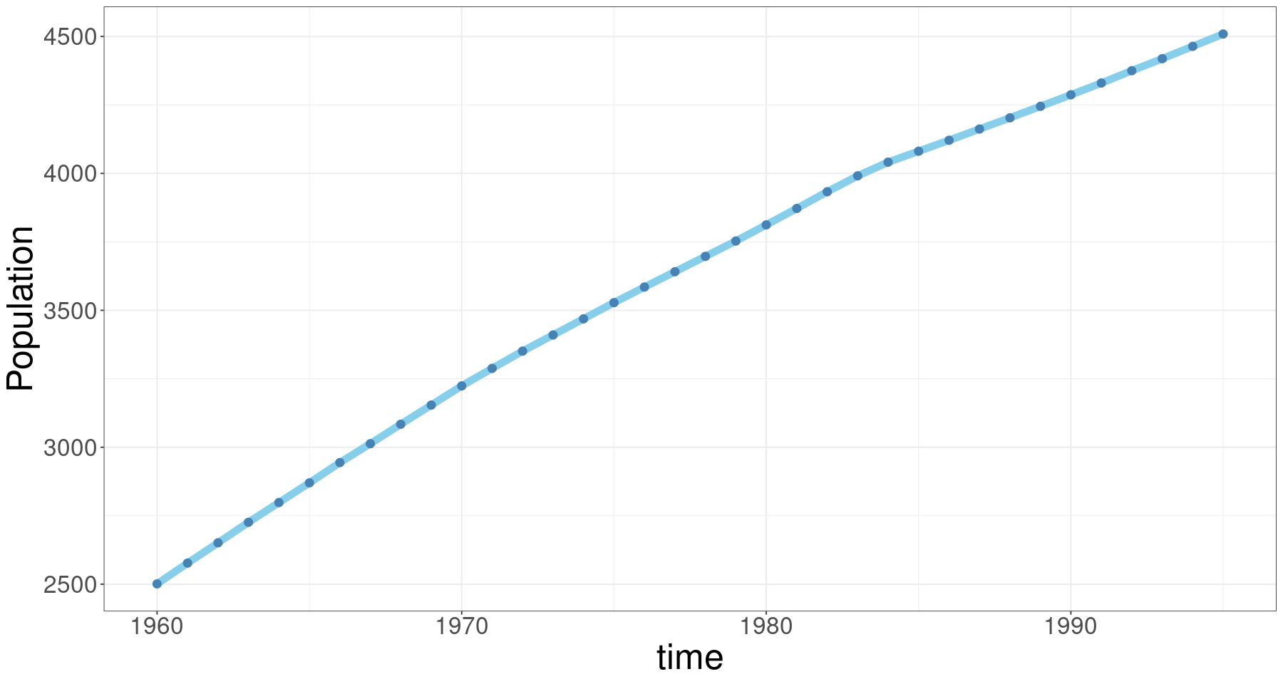
1차 선형 추세 모형
\[\text{모형}: Z_t = \beta_0 + \beta_1 t + \epsilon_t, t=1,\dots, n\]
m1 <- lm(pop~t, data=tmp.data)
summary(m1)
Call:
lm(formula = pop ~ t, data = tmp.data)

Residuals:
    Min      1Q  Median      3Q     Max
-115.40  -48.30   16.87   54.37   63.29

Coefficients:
             Estimate Std. Error t value Pr(>|t|)
(Intercept) 2559.3889    20.0385  127.72   <2e-16 ***
t             57.0135     0.9444   60.37   <2e-16 ***
---
Signif. codes:  0 ‘***’ 0.001 ‘**’ 0.01 ‘*’ 0.05 ‘.’ 0.1 ‘ ’ 1

Residual standard error: 58.87 on 34 degrees of freedom
Multiple R-squared:  0.9908,    Adjusted R-squared:  0.9905
F-statistic: 3644 on 1 and 34 DF, p-value: < 2.2e-16plot(pop~day, tmp.data,
main = 'Population : observation vs. fitted value',
xlab="", ylab="",
type='l',
col='skyblue',
lwd=2, cex.axis=2, cex.main=2) +
points(pop~day, tmp.data, col="steelblue", cex=2, pch=16) +
lines(tmp.data$day, fitted(m1), col='red', lty=2, lwd=2)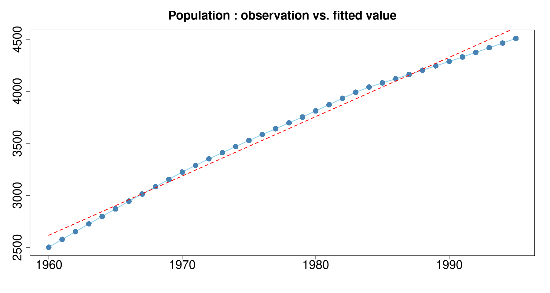
잔차분석
plot(tmp.data$day, resid(m1),
     pch=16, cex=2, xaxt='n',
     xlab="", ylab="", main="residual plot", cex.main=2)
abline(h=0, lty=2, lwd=2)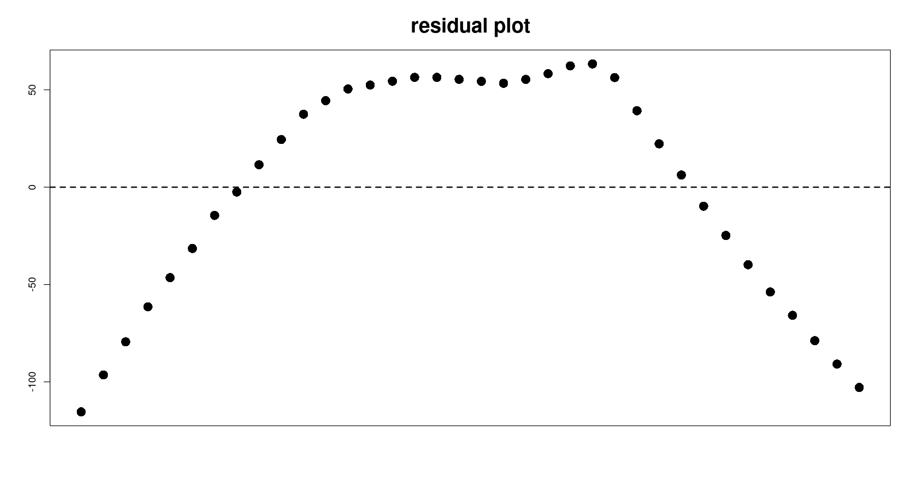
독립성검정(DW test)
dwtest(m1)
    Durbin-Watson test

data:  m1
DW = 0.041645, p-value < 2.2e-16
alternative hypothesis: true autocorrelation is greater than 0- 아무 옵션이 없으면 0보다 크냐는게 기본!! 대립가설확인필요
dwtest(m1, alternative="two.sided")
    Durbin-Watson test

data:  m1
DW = 0.041645, p-value < 2.2e-16
alternative hypothesis: true autocorrelation is not 0- 양측검정
dwtest(m1, alternative="less")
    Durbin-Watson test

data:  m1
DW = 0.041645, p-value = 1
alternative hypothesis: true autocorrelation is less than 0
정규분포 검정(shapro-wilk test)
- 가설
\(H_0\): 정규분포를 따른다. VS \(H_1\): 정규분포를 따르지 않는다.
hist(resid(m1))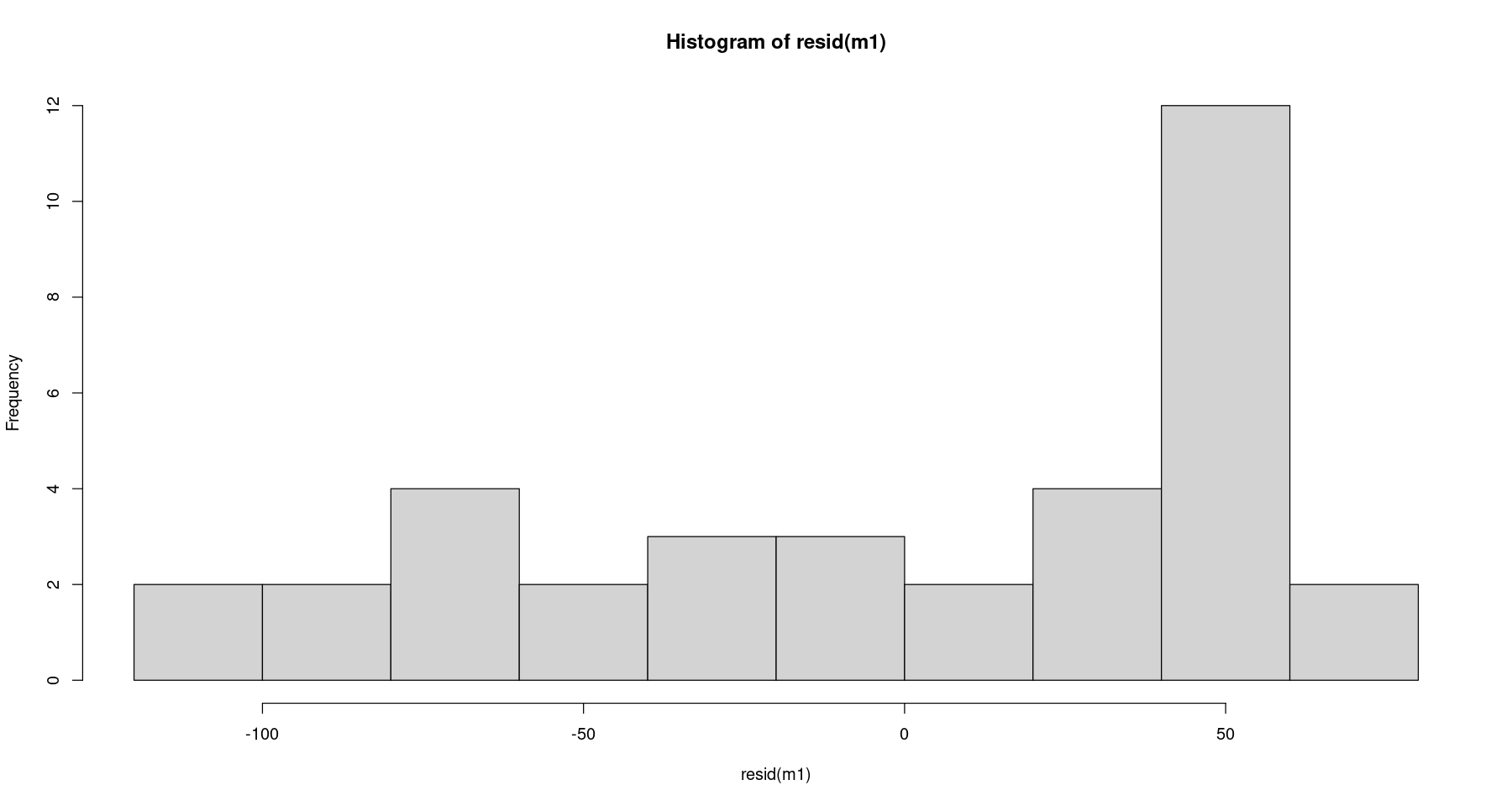
- 왼쪽으로 치우쳐져 있는 그림. 정규분포가 아닐거 같다.
shapiro.test(resid(m1)) #H_0 : 정규분포를 따른다.
    Shapiro-Wilk normality test

data:  resid(m1)
W = 0.87284, p-value = 0.000669
등분산성검정(Breusch–Pagan test)
- 가설
\(H_0\): 등분산 VS \(H_1\): 이분산
bptest(m1)
    studentized Breusch-Pagan test

data:  m1
BP = 0.0059664, df = 1, p-value = 0.9384
잔차에 대한 bptest를 한다. 위에 shapiro는 resid(m1)해줬지만 bptest는 그냥 바로 넣어 주면 된다.
pvalue값이 엄청 커서 기각 못함. 즉 등분산이다.
2차 선형 추세
\[\text{모형}: Z_t = \beta_0 + \beta_1 t + \beta_2 t^2 + \epsilon_t, t=1,\dots, n\]
m2 <- lm(pop~t+t2, data=tmp.data)
summary(m2)
Call:
lm(formula = pop ~ t + t2, data = tmp.data)

Residuals:
    Min      1Q  Median      3Q     Max
-11.365  -4.779  -1.049   3.798  17.631

Coefficients:
              Estimate Std. Error t value Pr(>|t|)
(Intercept) 2421.49090    4.05820  596.69   <2e-16 ***
t             78.78688    0.50576  155.78   <2e-16 ***
t2            -0.58847    0.01326  -44.38   <2e-16 ***
---
Signif. codes:  0 ‘***’ 0.001 ‘**’ 0.01 ‘*’ 0.05 ‘.’ 0.1 ‘ ’ 1

Residual standard error: 7.67 on 33 degrees of freedom
Multiple R-squared:  0.9998,    Adjusted R-squared:  0.9998
F-statistic: 1.083e+05 on 2 and 33 DF, p-value: < 2.2e-16- t2말고 \(I(t^2)\)으로 작성해줘도 된다. 대신 \(t^2\)으로 하게 되면 오류가 나니까 I지시함수 꼭 써주기
plot(pop~day, tmp.data,
 main = 'Population : observation vs. fitted value',
 xlab="", ylab="",
 type='l',
 col='skyblue',
 lwd=2, cex.axis=2, cex.main=2) +
 points(pop~day, tmp.data, col="steelblue", cex=2, pch=16) +
 lines(tmp.data$day, fitted(m2), col='red', lty=2, lwd=2)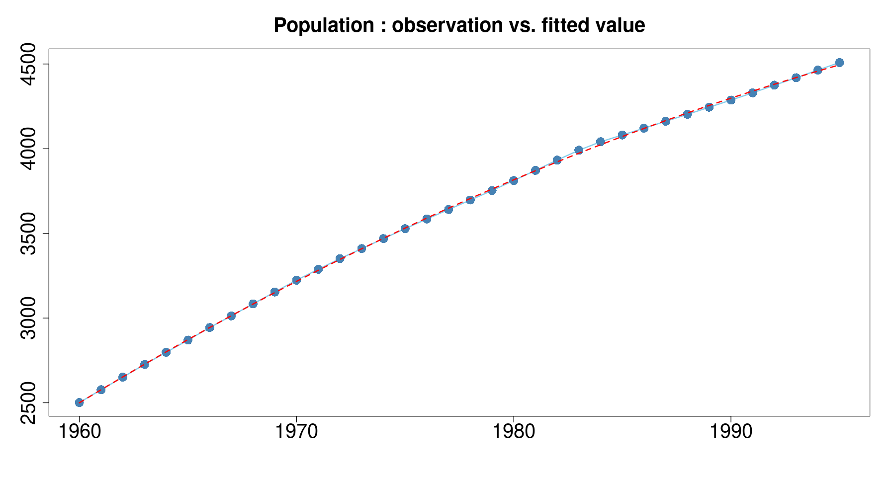
잔차분석
plot(tmp.data$day, resid(m2),
 pch=16, cex=2, xaxt='n',
 xlab="", ylab="", main="residual plot", cex.main=2)
abline(h=0, lty=2, lwd=2)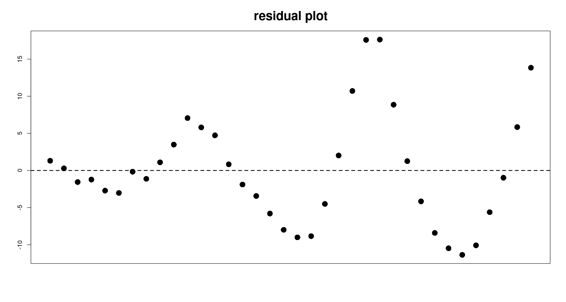
독립성 검정(DW test)
dwtest(m2,alternative = "two.sided")
    Durbin-Watson test

data:  m2
DW = 0.31083, p-value = 1.744e-13
alternative hypothesis: true autocorrelation is not 0dwtest(m2,alternative = "greater")
    Durbin-Watson test

data:  m2
DW = 0.31083, p-value = 8.72e-14
alternative hypothesis: true autocorrelation is greater than 0
정규성 검정
qqnorm(resid(m2), pch=16, cex=2)
qqline(resid(m2), col = 2, lwd=2)
hist(resid(m2))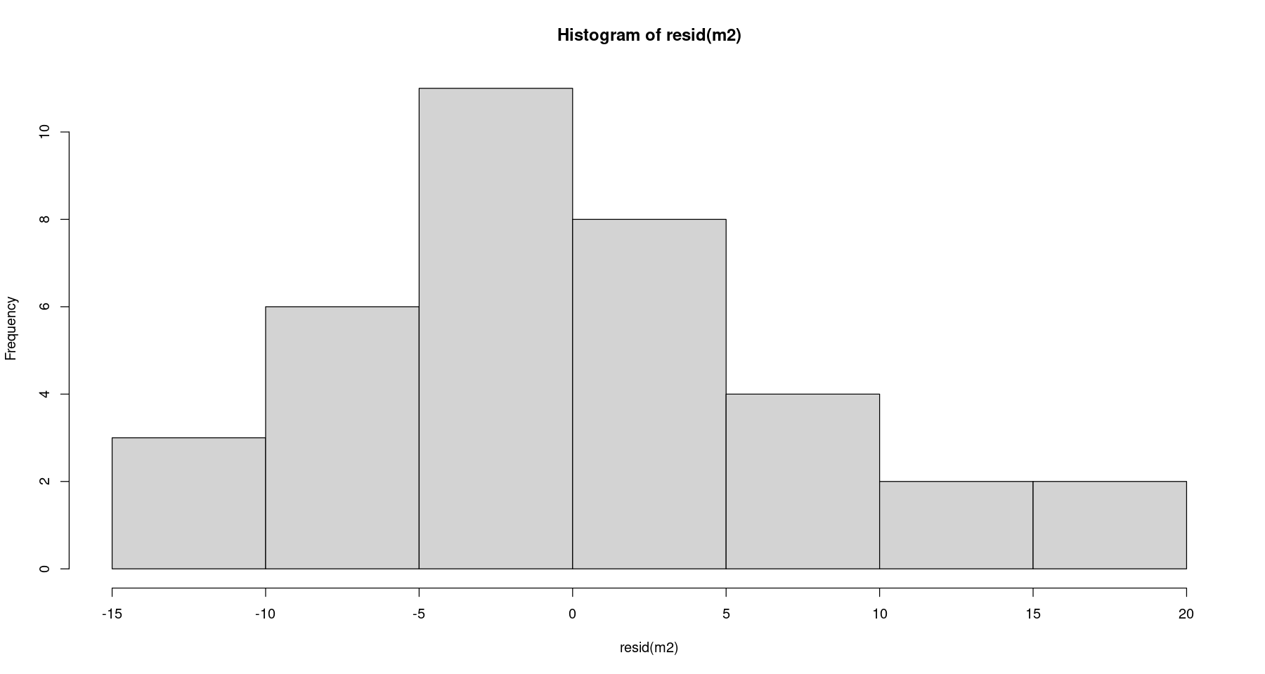
shapiro.test(resid(m2)) ##shapiro-wilk test
    Shapiro-Wilk normality test

data:  resid(m2)
W = 0.94947, p-value = 0.1007
등분산성 검정
bptest(m2)
    studentized Breusch-Pagan test

data:  m2
BP = 8.2455, df = 2, p-value = 0.0162- 이분산성이다.
로그변환 후 2차 추세
\[\text{모형}: ln(Z_t) = \beta_0 + \beta_1 t + \beta_2 t^2 + \epsilon_t, t=1,\dots, n\]
m3 <- lm(log(pop)~t+t2, data=tmp.data)
summary(m3)
Call:
lm(formula = log(pop) ~ t + t2, data = tmp.data)

Residuals:
      Min        1Q    Median        3Q       Max
-0.009306 -0.003520 -0.000374  0.003284  0.010159

Coefficients:
              Estimate Std. Error t value Pr(>|t|)
(Intercept)  7.807e+00  2.360e-03 3307.25   <2e-16 ***
t            2.740e-02  2.942e-04   93.14   <2e-16 ***
t2          -3.004e-04  7.712e-06  -38.95   <2e-16 ***
---
Signif. codes:  0 ‘***’ 0.001 ‘**’ 0.01 ‘*’ 0.05 ‘.’ 0.1 ‘ ’ 1

Residual standard error: 0.004461 on 33 degrees of freedom
Multiple R-squared:  0.9994,    Adjusted R-squared:  0.9993
F-statistic: 2.664e+04 on 2 and 33 DF, p-value: < 2.2e-16plot(log(pop)~day, tmp.data,
main = 'Population : observation vs. fitted value',
xlab="", ylab="",
type='l',
col='skyblue',
lwd=2, cex.axis=2, cex.main=2) +
points(log(pop)~day, tmp.data, col="steelblue", cex=2, pch=16) +
lines(tmp.data$day, fitted(m3), col='red', lty=2, lwd=2)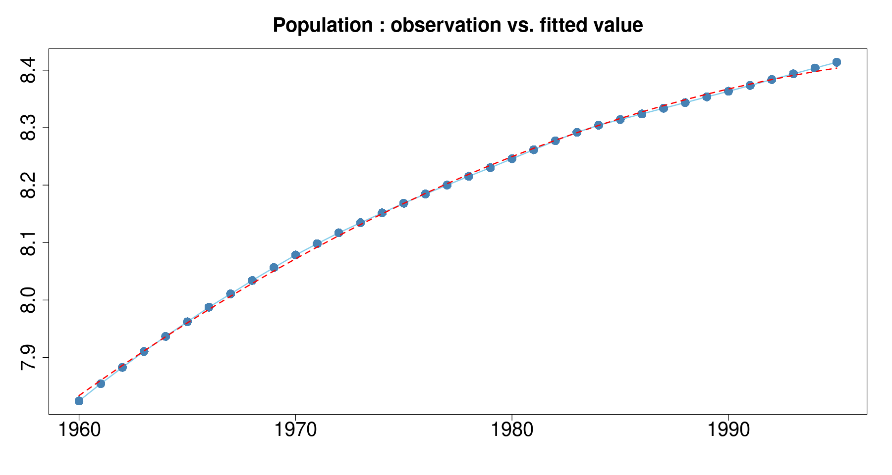
plot(pop~day, tmp.data,
 main = 'Population : observation vs. fitted value',
 xlab="", ylab="",
 type='l',
 col='skyblue',
 lwd=2, cex.axis=2, cex.main=2) +
 points(pop~day, tmp.data, col="steelblue", cex=2, pch=16) +
 lines(tmp.data$day, exp(fitted(m3)), col='red', lty=2, lwd=2)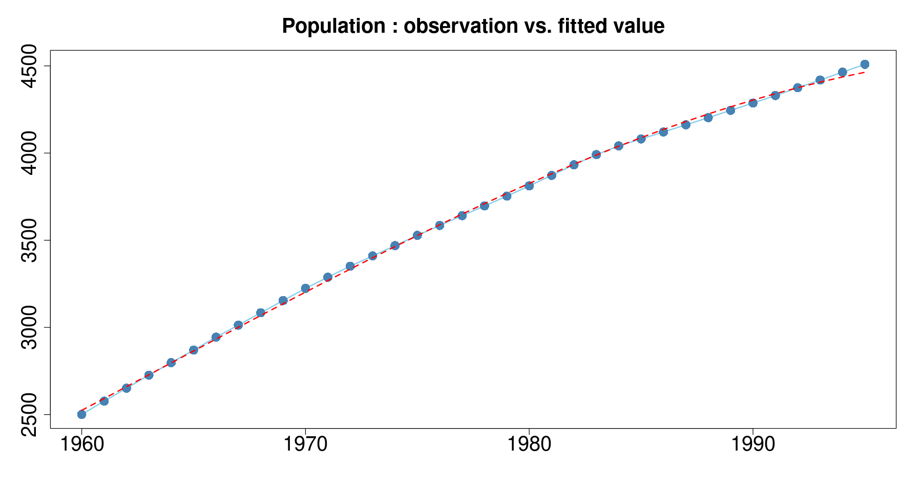
잔차분석
plot(tmp.data$day, resid(m3),
 pch=16, cex=2, xaxt='n',
 xlab="", ylab="", main="residual plot", cex.main=2)
abline(h=0, lty=2, lwd=2)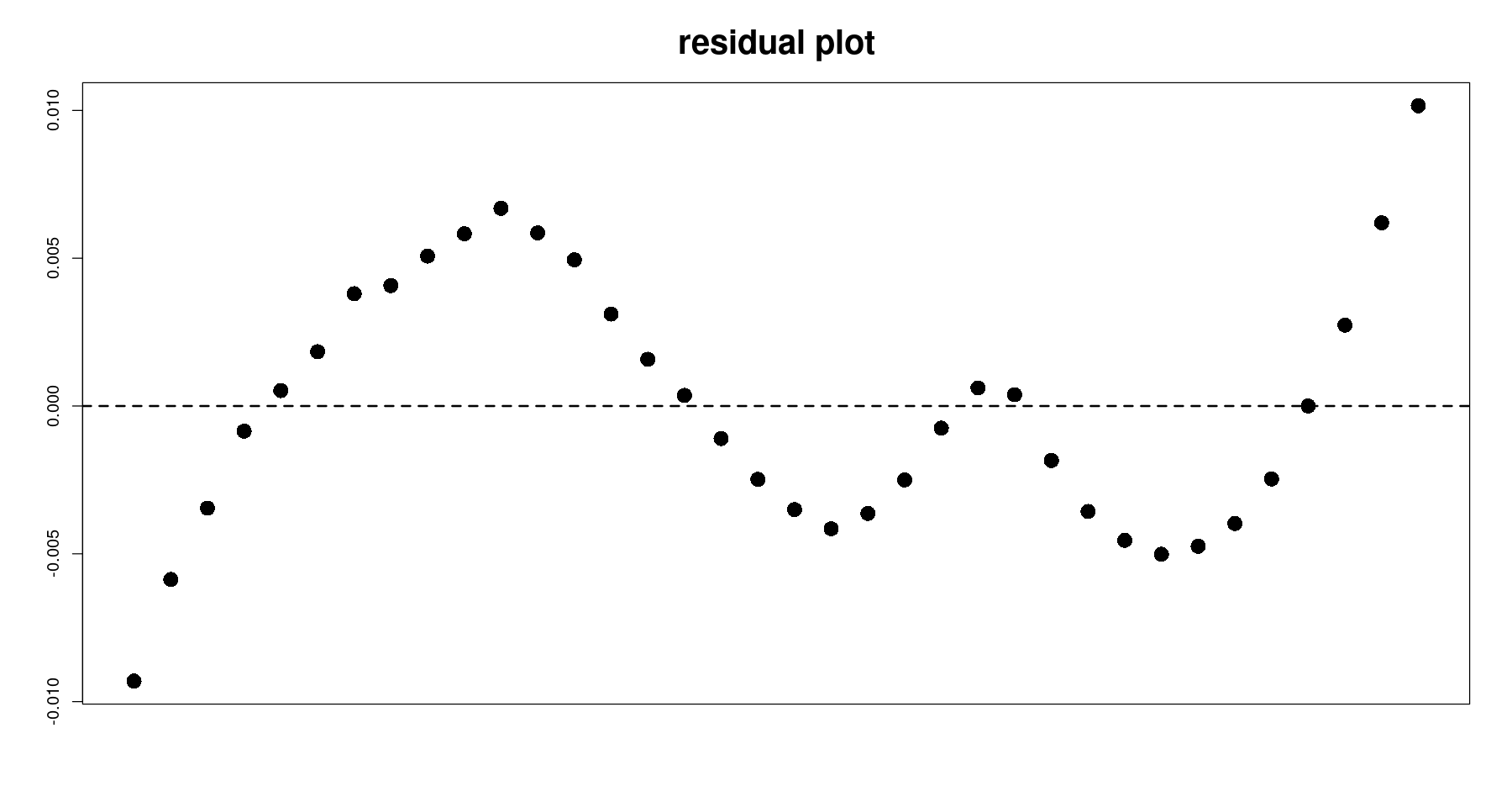
독립성 검정
dwtest(m3,alternative = "two.sided")
    Durbin-Watson test

data:  m3
DW = 0.16493, p-value < 2.2e-16
alternative hypothesis: true autocorrelation is not 0dwtest(m3,alternative = "greater")
    Durbin-Watson test

data:  m3
DW = 0.16493, p-value < 2.2e-16
alternative hypothesis: true autocorrelation is greater than 0
정규성 검정
qqnorm(resid(m2), pch=16, cex=2)
qqline(resid(m2), col = 2, lwd=2)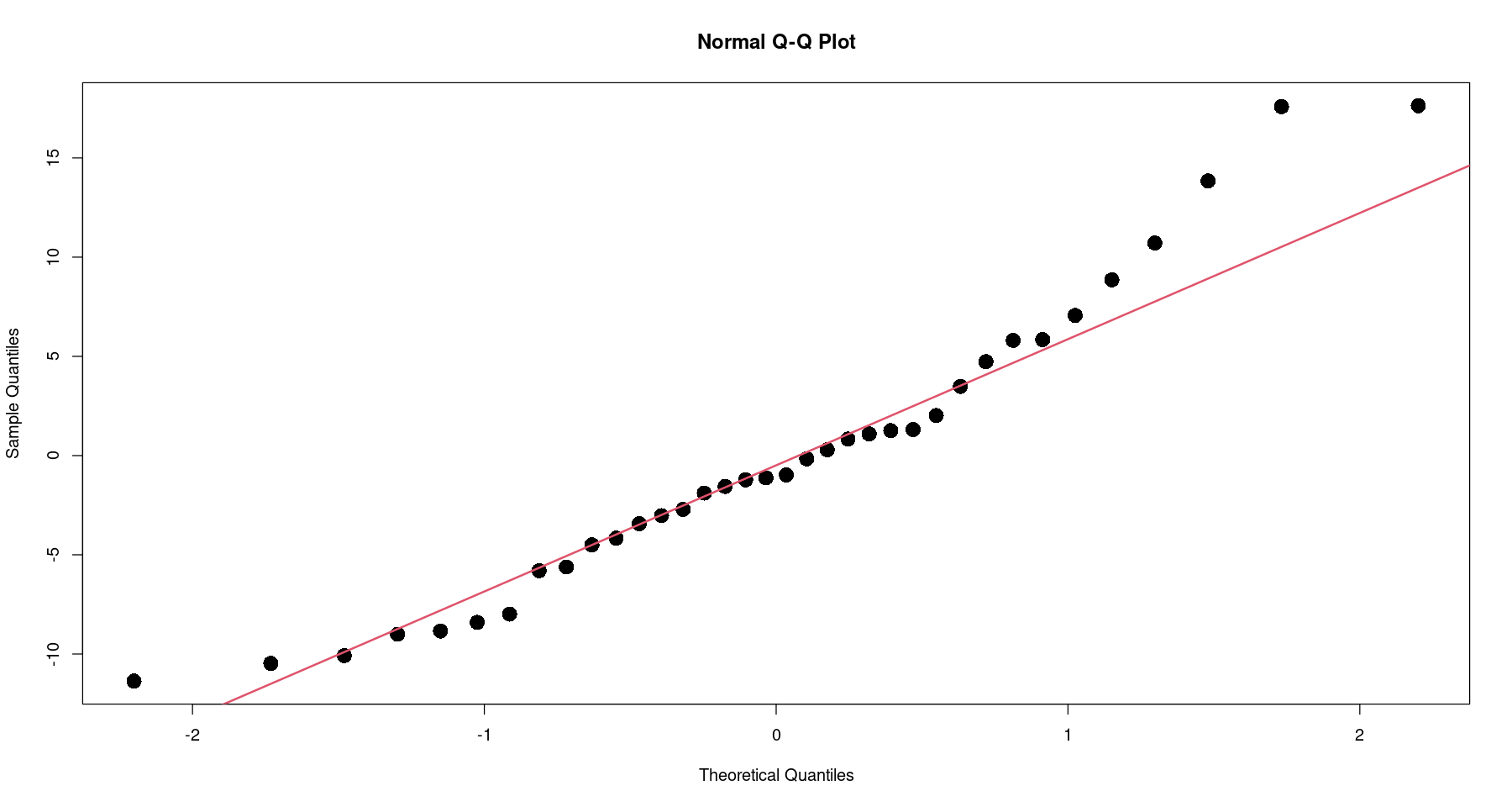
hist(resid(m3))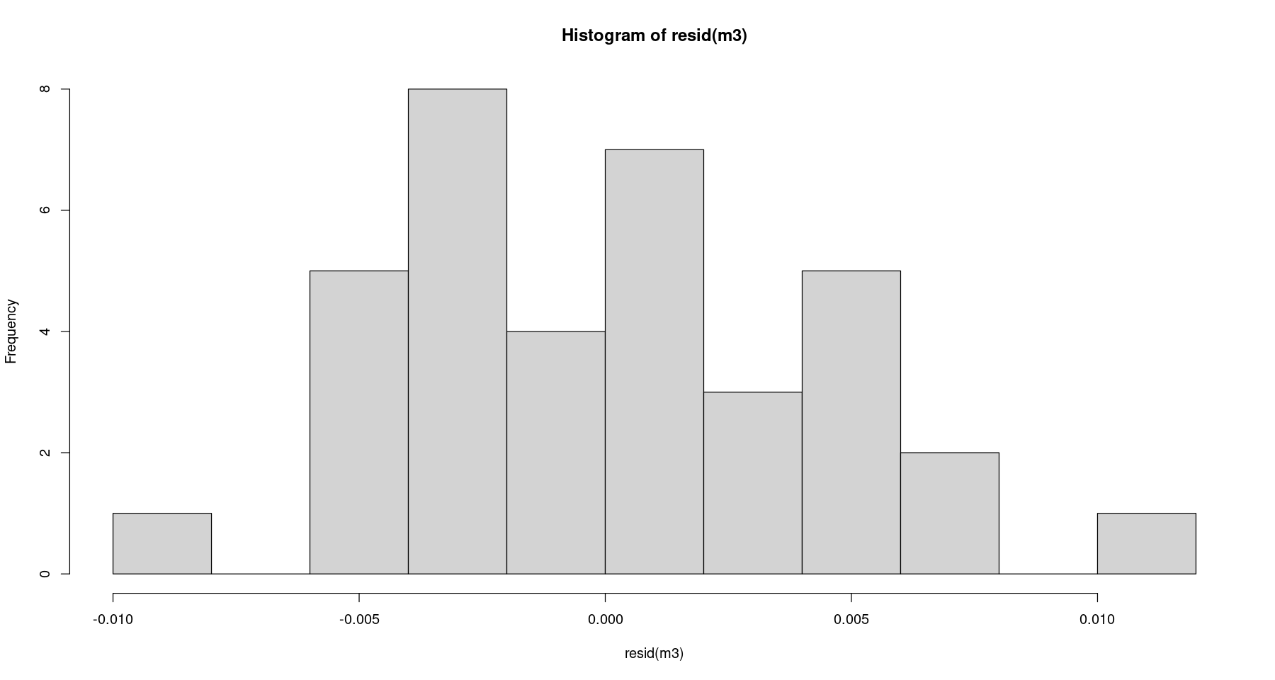
shapiro.test(resid(m3))
    Shapiro-Wilk normality test

data:  resid(m3)
W = 0.97547, p-value = 0.5922
등분산성 검정
bptest(m3)
    studentized Breusch-Pagan test

data:  m3
BP = 8.8866, df = 2, p-value = 0.01176